-
Notifications
You must be signed in to change notification settings - Fork 117
Super Time Stepping
Explicit integration of diffusive physics requires taking a parabolic time-step, which is proportional to , where
is the linear resolution of the calculation. This parabolic time-step is often much smaller than the hyperbolic time-step, thus dramatically increasing the required compute time when running Athena++ with diffusive physics enabled.
Super-time-stepping offers an avenue to alleviate some of the penalty associated with an explicit scheme. When super-time-stepping is enabled, diffusive physics is treated in an operator-split fashion using the RKL algorithm (see Meyer et al. 2014). Athena++ has available the first-order accurate RKL1 integrator (sts_integrator=rkl1) and the second order accurate RKL2 integrator (sts_integrator=rkl2). These integrators enable us to take the hyperbolic time-step inside the main integration loop, while diffusive physics is integrated using super-time-steps. A super-time-step is comprised of s stages where
Above, a and b are constants that depend on STS integrator choice. , is the super-time-step, equal to the hyperbolic time-step in the RKL1 integrator, or half the hyperbolic time-step in the RKL2 integrator. Thus, one can see that for the RKL1 integrator, one operator split super-time-step is needed to integrate diffusive physics forward by one hyperbolic time-step. Similarly, for the RKL2 integrator, two operator split super-time-steps are needed (one taken before main integration, one after) to integrate diffusive physics forward by one hyperbolic time-step.
The larger the ratio between the hyperbolic and parabolic time-step, the larger the value of s. The speedup associated with super-time-stepping is proportional to s.
Super-time-stepping can only be applied to problems with diffusive physics. To enable super-time-stepping, configure Athena++ with the -sts option.
> python configure.py -sts
If super-time-stepping is enabled, at least one of the following input parameters for diffusion processes must be set in the input file under the <problem> block:
    <problem>
    nu_iso      = 0.01       # isotropic viscosity coefficient
    nu_aniso    = 0.0        # anisotropic viscosity coefficient
    kappa_iso   = 0.01       # isotropic thermal conduction coefficient
    kappa_aniso = 0.0        # anisotropic thermal conduction coefficient
    eta_ohm     = 0.01       # Ohmic resistivity coefficient
    eta_ad      = 0.0        # Ambipolar diffusion coefficient
There are several optional parameters that can be set in the input file under the <time> block:
    <time>
    sts_integrator = rkl1   # sts integration algorithm
    dt_diagnostics = -1     # extra timestep diagnostic info
    sts_max_dt_ratio = -1   # max dt to parabolic dt ratio
-
sts_integrator(optional) : sts integration algorithm. Choices:-
rkl1: first-order accurate RKL1 algorithm -
rkl2(default) : second-order accurate RKL2 algorithm
-
-
dt_diagnostics(optional) : output extra timestep diagnostic info to stdout (at everyncycle_outinterval). Choices:-
-1(default) : disabled -
0: listdt_hyperbolic,dt_parabolic, anddt_user(if active) and their respective ratios to the overall main integratordt. With STS enabled, the following metric is also output:stage_ratio = (dt*nstages)/(dt_parabolic*(nstages + nstages_sts)), wherenstagescorresponds to the main multistage explicit time-integrator. -
n= positive integer : same behavior as0, but output extra diagnostics at every STS stage for proof-of-progress if-stswas used during Configuring.
-
-
sts_max_dt_ratio(optional) : limit time-step if the ratio of overalldttodt_parabolicexceeds this value (-1 = infinity = default)
Ohmic diffusion of a Gaussian magnetic field:
> python configure.py -b -sts --prob=resist --eos=isothermal
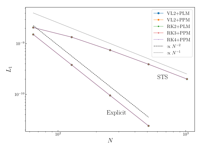
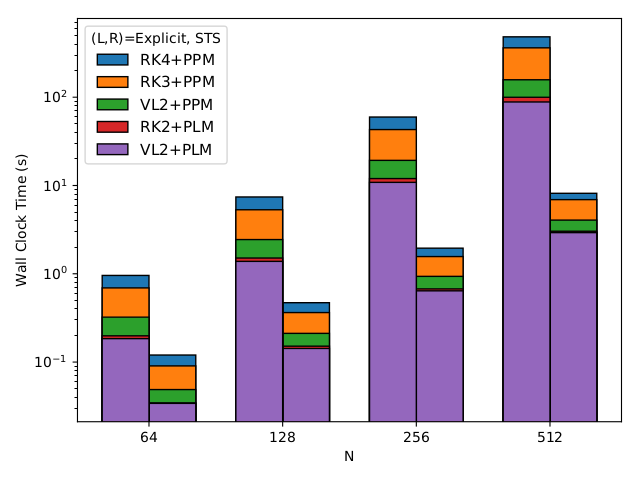
Error convergence and performance diagnostics for RKL1 super-time-stepping vs. explicit integration in the Ohmic diffusion example problem:


- For diffusion problems with very large
dttodt_parabolicratios, super-time-stepping accuracy begins to diminish. Although very problem/physics/resolution dependent, we advise users to enrollsts_max_dt_ratioin cases where such behavior is seen. In our experience,sts_max_dt_ratio=100adequately throttles super-time-stepping, however, we strongly encourage users to test and use caution. - If enrolling user-defined source terms with STS, note that
fluxcontains only non-diffusive fluxes. - When using orbital advection with STS,
orbital_advection/OAorder=2andtime/sts_integrator=rkl2are recommended.
Getting Started
User Guide
- Configuring
- Compiling
- The Input File
- Problem Generators
- Boundary Conditions
- Coordinate Systems and Meshes
- Running the Code
- Outputs
- Using MPI and OpenMP
- Static Mesh Refinement
- Adaptive Mesh Refinement
- Load Balancing
- Special Relativity
- General Relativity
- Passive Scalars
- Shearing Box
- Diffusion Processes
- General Equation of State
- FFT
- High-Order Methods
- Super-Time-Stepping
- Orbital Advection
- Rotating System
- Reading Data from External Files
Programmer Guide