There are two variants for setting up a Barefoot map server. The first variant uses an easy-to-use Docker container ('blue pill' - recommended in almost every case). The other variant enables you to set up a map server within an existing PostgreSQL/PostGIS server ('red pill' - self-maintained database).
The following approach uses Docker (version 1.6 or higher, see here) to automatically install PostgreSQL/PostGIS database server in an isolated container environment. With simple scripts an OpenStreetMap extract can be easily imported into the database.
- Build Docker image.
cd barefoot
sudo docker build --rm=true -t barefoot ./docker- Create Docker container.
Note: Give the container a name by replacing <container> respectively.
sudo docker run -t -i -p 127.0.0.1:5432:5432 --name="<container>" -v ${PWD}/bfmap/:/mnt/bfmap -v ${PWD}/docker/osm/:/mnt/osm barefoot- Import OSM extract (in the container).
root@acef54deeedb# bash /mnt/osm/import.sh <osm> <database> <user> <password> <config> slim|normal- To import an OpenStreetMap extract
<osm>put the file in the directorydocker/osmfrom outside the container which is then accessible inside the container at/mnt/osm/. - The script imports the extract into a database with specified name and credentials, i.e.
<database>,<user>, and<password>. - A road type specification
<config>must be provided as path to a file with the specification in JSON format. An example is included atbfmap/road-types.json. - Standard import mode
normalexecutes a bunch of SQL queries to import OSM data extract of any size, whereasslimmode runs the import in a single query which is fast but requires lots of memory. The latter should be used only for small OSM data extracts (extracts of at most the size of e.g. Switzerland).
Note: To detach the interactive shell from a running container without stopping it, use the escape sequence Ctrl-p + Ctrl-q.
The test map server setup follows the standard setup but uses a pre-configured import script.
- Download OSM extract (examples require
oberbayern.osm.pbf)
curl http://download.geofabrik.de/europe/germany/bayern/oberbayern-latest.osm.pbf -o barefoot/docker/osm/oberbayern.osm.pbf- Build Docker image (if not done yet).
cd barefoot
sudo docker build --rm=true -t barefoot ./docker- Create Docker container.
sudo docker run -t -i -p 127.0.0.1:5432:5432 --name="barefoot-oberbayern" -v ${PWD}/bfmap/:/mnt/bfmap -v ${PWD}/docker/osm/:/mnt/osm barefoot- Import OSM extract (in the container) with default parameters.
root@acef54deeedb# bash /mnt/osm/import.shSome general commands for administration of the Docker container:
- Start/stop container:
sudo docker start sudo docker stop
- Attach to container (for maintenance):
``` bash
sudo docker attach <container>
root@acef54deeedb# sudo -u postgres psql -d <database>
psql (9.3.5)
Type "help" for help.

<database>=# \q
root@acef54deeedb#
Note: To detach the interactive shell from a running container without stopping it, use the escape sequence Ctrl-p + Ctrl-q.
- Show containers:
$ sudo docker ps -a CONTAINER ID IMAGE COMMAND CREATED STATUS PORTS NAMES acef54deeedb -image:latest /bin/sh -c 'service 3 minutes ago Up 2 seconds 127.0.0.1:5432->5432/tcp
#### Test import scripts

_Note: This is only useful, if you work on the Python import scripts._

1. Build Docker image (if not done yet).

``` bash
cd barefoot
sudo docker build --rm=true -t barefoot ./docker
- Create test container.
sudo docker run -t -i -p 127.0.0.1:5432:5432 --name="barefoot-test" -v ${PWD}/bfmap/:/mnt/bfmap -v ${PWD}/docker/osm/:/mnt/osm barefoot- Run test script (in the container).
root@8160f9e2a2c0# bash /mnt/bfmap/test/run.shNote: Currently, there is no support for compiling a barefoot map from XML-based OSM data directly (*.osm or *.osm.pbf files). Hence, it is necessary to use Osmosis as shown in the following steps.
- Install prerequisites.
- PostgreSQL (version 9.3 or higher)
- PostGIS (version 2.1 or higher)
- Osmosis (versionb 0.43.1 or higher)
- Python (version 2.7.6 or higher)
- Psycopg2
- NumPy
- Python-GDAL
- Setup the database and include extensions.
createdb -h <host> -p <port> -U <user> <database>
psql -h <host> -p <port> -U <user> -d <database> -c "CREATE EXTENSION postgis;"
psql -h <host> -p <port> -U <user> -d <database> -c "CREATE EXTENSION hstore;"-
Import the OSM data.
-
Download and set up OSM database schema.
``` bash
wget https://trac.openstreetmap.org/export/22680/subversion/applications/utils/osmosis/trunk/package/script/pgsql_simple_schema_0.6.sql psql -h -p -U -d -f pgsql_simple_schema_0.6.sql ```
- Import OSM extract with osmosis.
``` bash
osmosis --read-pbf file=<osm.pbf-file> --write-pgsql host=: user= database= password= ```
 __Note:__ In some cases, it is necessary to specify to a temporary directory to be used by osmosis. (This is necessary for example if osmosis stops with error 'No space left on device'.) To do so, run the following commands beforehand:

 ``` bash
JAVACMD_OPTIONS=-Djava.io.tmpdir= export JAVACMD_OPTIONS ```
- Extract OSM ways in intermediate table.
Usually, you can run the import in slim mode, which creates the table <ways-table> in a single query:
bfmap/osm2ways --host <host> --port <port> --database <database> --table <ways-table> --user <user> --slimHowever, if memory is not sufficiently available, use normal mode. This requires to specify a prefix <prefix> for temporary tables. This prevents deleting and overwriting existing tables:
bfmap/osm2ways --host <host> --port <port> --database <database> --table <ways-table> --user <user> --prefix <prefix>Note: To see what the commands are doing, you can add the option --printonly to see the SQL commands to be executed.
- Compile Barefoot map data.
Transform ways table <ways-table> into routing table <bfmap-table>. The configuration <config>, use e.g. bfmap/road-types.xml
bfmap/ways2bfmap --source-host <host> --source-port <port> --source-database <host> --source-table <ways-table> --source-user <user> --target-host <host> --target-port <port> --target-database <database> --target-table <bfmap-ways> --target-user <user> --config <config>Note: To see what the commands are doing, you can add the option --printonly to see the SQL commands to be executed.
-
Setup a map server, see here.
-
Assemble Barefoot JAR with dependencies. (Includes the executable main class of the server.)
cd barefoot
mvn compile assembly:single- Start map matching server.
A map matching server is a Java process that is accessible via TCP/IP socket and requires configuration for access to the map server and settings of the map matching server.
java -jar target/barefoot-0.0.2-jar-with-dependencies.jar [--slimjson|--debug|--geojson] /path/to/server/properties /path/to/mapserver/properties-
Map server properties contains access information to map server.
Note: An example is included at
config/oberbayern.propertieswhich can be used as reference or for testing. -
Server properties contains configuration for the server and map matching. Settings for configuration are explained below.
Note: An example is included at
config/server.propertiesand can be used for testing. The details for parameter settings are shown below.
A map matching request is sent to the server via TCP/IP connection. For simple testing, netcat can be used to send requests. An example request is included at src/test/resources/com/bmwcarit/barefoot/matcher/x0001-015.json.
cat src/test/resources/com/bmwcarit/barefoot/matcher/x0001-015.json | netcat 127.0.0.1 1234A map matching request is a text message with a JSON array of JSON objects in the following form:
[
	{"id":"a1396ab7-7caa-4c31-9f3c-8982055e3de6","time":1410324847000,"point":"POINT (11.564388282625075 48.16350662940509)"},
	...
]idis user-specific identifier and has no further meaning for map matching or the server.timeis a timestamp in milliseconds unix epoch time.pointis a position (measurement) in WKT (well-known-text) format and with WGS-84 projection (SRID 4326). (In other words, this may be any GPS position in WKT format.)
Default response format is the JSON representation of the k-state data structure, see k-State data structure. To change default output format, use the following options:
--slimjson: Server outputs JSON format with map matched positions, consisting of road id and fraction as precise position on the road, and routes between positions as sequences of road ids.--debug: Server outputs a JSON format similar to slim JSON format, but with timestamps of the measurements and geometries of the routes in WKT format.--geojson: Server outputs the geometry of the map matching on the map in GeoJSON format.
A request may demand another response format by encapsulating the request in a JSON object of the form:
{
	"format": "<format>",
	"request": <request>
}
For example, a request using netcat may be as follows:
echo "{\"format\": \"geojson\", \"request\": $(cat src/test/resources/com/bmwcarit/barefoot/matcher/x0001-015.json | tr -d '\n\r')}" | netcat 127.0.0.1 1234The server properties includes configuration of the server, e.g. TCP/IP port number, number of threads, etc., and parameter settings of the map matching.
| Parameter | Default value | Description |
|---|---|---|
| portNumber | 1234 | The port of the map matching server. |
| maxRequestTime | 15000 | Maximum time in milliseconds of waiting for a request after connection has been established. |
| maxResponseTime | 60000 | Maximum time in milliseconds of waiting for reponse processing before a timeout is triggered and processing is aborted. |
| maxConnectionCount | 20 | Maximum number of connections to be established by clients. |
| numExecutorThreads | 40 | Number of executor threads for reponse handling (I/O), which should be a multiple of the number of processors/cores of the machine to fully exploit the machine's performance. |
| matcherSigma | 5 | Standard deviation of the position measurement error in meters, which is usually 5 meters for standard GPS error, as probability measure of matching candidates for position measurements on the map. |
| matcherLambda | 0.0 | Rate parameter of negative exponential distribution for probability measure of routes between matching candidates. (The default is 0.0 which enables adaptive parameter setting, depending on sampling rate and input data, other values (manually fixed) may be 0.1, 0.01, 0.001 ...) |
| matcherMaxDistance | 15000 | Maximum length of routes to be searched in the map for transitions between matching candidates in meters. (This avoids searching the full map for candidates that are for some reason not connected in the map, e.g. due to missing road links.) |
| matcherMaxRadius | 200 | Maximum radius for matching candidates to be searched in the map for respective position measurements in meters. |
| matcherMinInterval | 5000 | Minimum time interval in milliseconds for measurements to be considered for matching. Any measurement taken in less than the minimum interval after the most recent measurement is skipped. (This avoids unnnecessary matching of positions with very high measuremnt rate, useful e.g. if the measurement rate varies.) |
| matcherMinDistance | 10 | Minimum distance in meters for measurements to be considered for matching. Any measurement taken in less than the minimum distance from the most recent measurement is skipped. (This avoids unnnecessary matching of positions with very high measurement rate, useful e.g. if the object speed varies.) |
| matcherNumThreads | 8 | Number of executor threads for reponse processing (map matching), which should at least the number of processors/cores of the machine to fully exploit the machine's performance. |
Note: Barefoot library requires Java 7 or higher.
- Add dependency to your Java project with Maven:
<dependency>
  	<groupId>de.bmw-carit.barefoot</groupId>
  	<artifactId>barefoot</artifactId>
  	<version>0.0.2</version>
</dependency>- Set up a map server, see here.
Note: Use this approach only if Barefoot is not available with a public Maven repository.
- Checkout the respository.
git clone https://github.com/bmwcarit/barefoot.git
cd barefoot- Install JAR to your local Maven repository.
Note: Maven tests will fail if the test map server hasn't been setup as shown here.
mvn install... and to skip tests (if test map server has not been set up) ...
mvn install -DskipTests- Add dependency to your Java project with Maven.
<dependency>
  	<groupId>com.bmw-carit</groupId>
  	<artifactId>barefoot</artifactId>
  	<version>0.0.2</version>
</dependency>- Set up a map server, see here.
mvn javadoc:javadocSee here.
A Hidden Markov Model (HMM) assumes that a system's state is only observable indirectly via measurements over time. This is the same in map matching where a sequence of position measurements (trace), recorded e.g with a GPS device, contains implicit information about an object's movement on the map, i.e. roads and turns taken. Hidden Markov Model (HMM) map matching is a robust method to infer stochastic information about the object's movement on the map, cf. [1] and [2], from measurements and system knowledge that includes object state candidates (matchings) and its transitions (routes).
A sequence of position measurements z0, z1, ..., zT is map matched by finding for each measurement zt, made at some time t (0 ≤ t ≤ T), its most likely matching on the map sti from a set of matching candidates St = {st1, ..., stn}. A set of matching candidates St is here referred to as a candidate vector. For each consecutive pair of candidate vectors St and St+1 (0 ≤ t < T), there is a transition between each pair of matching candidates sti and st+1j which is the route between map positions in the map. An illustration of the HMM with matching candidates and transitions is shown in the figure below.

To determine the most likely matching candidate, it is necessary to quantify probabilities of matching candidates and respective transitions. A HMM defines two types of probability measures:
- A position measurement is subject to error and uncertainty. This is quantified with an emission probability p(zt | st) that defines a conditioned probability of observing measurement zt given that the true position in the map is st, where p(zt | st) ∼ p(st | zt).
Here, emission probabilities are defined with the distance between measured positions to its true position is used to model measurement errors which is described with gaussian distribution with some standard deviation σ (default is σ = 5 meters).
-
All transitions between different pairs of matching candidates st-1 to st have some measure of plausiblity which is quantified with a transition probability p(st | st-1) that is a conditioned probability of reaching st given that st-1 is the origin.
Here, transition probabilities are quantified with the difference of routing distance and line of sight distance between respective position measurements. Transition probabilities are distributed negative exponentially with a rate parameter λ (default is λ = 0.1) which is the reciprocal of the mean.
In HMM map matching, we distinguish two different solutions to map matching provided by our HMM filter:
- Our HMM filter determines an estimate s̅t of the object's current position which is the most likely matching candidate st ∈ St given measurements z0 ... zt, which is defined as:
s̅t = argmax(st ∈ St) p(st|z0 ... zt),
where p(st|z0 ... zt) is referred to as the filter probability of st and can be determined recursively:
p(st|z0...zt) = p(st|zt) · Σ(st-1 ∈ St-1) p(st|st-1) · p(st-1|z0 ... zt-1).
-
In addition, we extend our HMM filter to determine an object's most likely path s0 ... sT, that is the most likely sequence of matching candidates st ∈ St given the full knowledge of measurements z0 ... zT, which is defined as:
s0 ... sT = argmax(sT ∈ ST) p(s0 ... sT|z0 ... zT),
where we define p(s0 ... st|z0 ... zt) as the probability of the most likely sequence that reaches matching candidate st, referred to as the sequence probability of st, and can be also determined recursively:
p(s0 ... st|z0 ... zt) = p(st|zt) · argmax(st-1 ∈ St-1) p(st|st-1) · p(s0 ... st-1|z0 ... zt-1).
Note: Here, p(s0 ... st|z0 ... zt) is defined as the probability of the most likely sequence that reaches candidate st, whereas in other literature, cf. [4], it is defined as the probability of the sequence s0 ... st. This is used for convenience to enable implementation of online and offline map matching in dynamic programming manner (according to online Viterbi algorithm). Nevertheless, the solution is the same.
Since both solutions are recursive both can be used for online and offline algorithms, i.e. online and offline map matching.
Barefoot's map matching API consists of four main components. This includes a matcher component that performs map matching with a HMM filter iteratively for each position measurement zt of an object. It also includes a state memory component that stores candidate vectors St and their probabilities p; and it can be accessed to get the current position estimate s̅t or the most likely path (s0 ... st). Further, it includes a map component for spatial search of matching candidates St near the measured position zt; and a router component to find routes ⟨st-1,st⟩ between pairs of candidates (st-1,st).
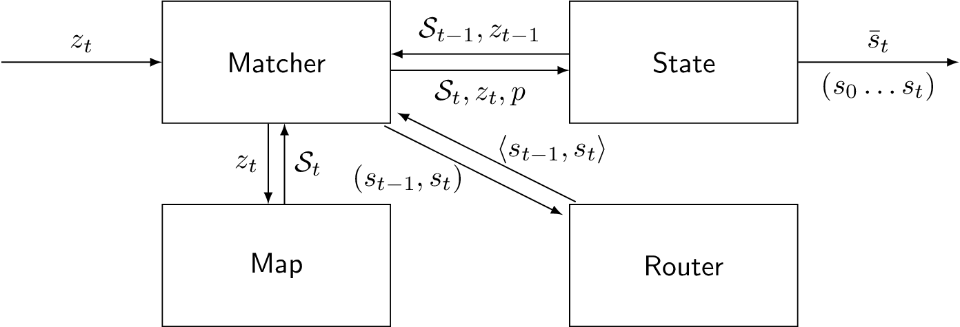
A map matching iteration is the processing of a position measurement zt to update the state memory and includes the following steps:
- Spatial search for matching candidates st ∈ St in the map given measurement zt. St is referred to as a candidate vector for time t.
- Fetch candidate vector St-1 from memory if there is a candidate vector for time t-1 otherwise it returns an empty vector.
- For each pair of matching candidates (st-1, st) with st-1 ∈ St-1 and st ∈ St, find the route ⟨st-1,st⟩ as the transition between matching candidates.
- Calculate filter probability and sequence probability for matching candidate st, and update state memory with probabilities p and candidate vector St.
A simple map matching program shows the use of the map matching API (for details, see the Javadoc):
import com.bmwcarit.barefoot.matcher.Matcher;
import com.bmwcarit.barefoot.matcher.KState;
import com.bmwcarit.barefoot.matcher.MatcherCandidate;
import com.bmwcarit.barefoot.matcher.MatcherSample;
import com.bmwcarit.barefoot.matcher.MatcherTransition;
import com.bmwcarit.barefoot.road.PostGISReader;
import com.bmwcarit.barefoot.roadmap.RoadMap;
import com.bmwcarit.barefoot.roadmap.Route;
import com.bmwcarit.barefoot.roadmap.TimePriority;
import com.bmwcarit.barefoot.spatial.Geography;
import com.bmwcarit.barefoot.topology.Dijkstra;

import com.esri.core.geometry.Point;

// Load and construct road map
RoadMap map = RoadMap.Load(new PostGISReader(...));
map.construct();

// Instantiate matcher and state data structure
Matcher matcher = new Matcher(map, new Dijkstra<Road, RoadPoint>(),
			new TimePriority(), new Geography());
KState<MatcherCandidate, MatcherTransition, MatcherSample> state =
			new KState<MatcherCandidate, MatcherTransition, MatcherSample>();

// Input as sample batch (offline) or sample stream (online)
List<MatcherSample> samples = new LinkedList<MatcherSample>();

// Iterative map matching of sample batch (offline) or sample stream (online)
for (MatcherSample sample : samples) {
	Set<MatcherCandidate> vector = matcher.execute(state.vector(), state.sample(),
			sample);
	state.update(vector, sample);

	// Online map matching result
	MatcherCandidate estimate = state.estimate(); // most likely position estimate

	long id = estimate.point().edge().id(); // road id
	Point position = estimate.point().geometry(); // position
	Route route = estimate.transition().route(); // route to position
}

// Offline map matching results
List<MatcherCandidate> sequence = state.sequence(); // most likely sequence of positionsA k-State data structure is a state memory for map matching. It organizes sets of matching candidates as candidate vectors, and provides access to:
- a matching estimate which is the most likely matching candidate s̅t for time t and represents an estimate of the object's current position on the map,
- and an estimate of the sequence which is the most likely sequence of matching candidates (s0 ... st) and represents the object's most likely path on the map.
The k-State data structure is initially empty and must be updated with state vectors St. After the first update with state vector S0 (left subfigure), it contains matching candidates (circles) with a pointer to the estimate (thick circle). In the second matching iteration (middle subfigure), the matcher fetches state vector S0 and determines for each matching candidate s1i ∈ S1 its sequence and filter probability, and determines the most likely predecessor candidate in S0 (black arrows). After that, state vector S1 is used to update the state memory (right subfigure) which, in turn, updates pointers to the estimate and the most likely sequence (thick arrow).


Each matching iteration repeats basically the same procedure: fetching state vector St-1 (left subfigure), calculating for each candidate st ∈ St filter and sequence probability and its most likely predecessor in St-1 (middle subfigure), and updating state memory (right subfigure). With every update the k-State data structure converges, i.e. it removes all matching candidates that are neither relevant to the estimate nor to the most likely sequence.


A k-State data structure provides two parameters to configure a maximum capacity in the number of state vectors stored in k-State (mostly relevant to online map matching):
- k bounds the number of state vectors to at most k+1 state vectors with k ≥ 0, i.e. state vectors St-k ... St. If k is negative it is unbounded.
- τ bounds the number of state vectors in time to only those state vectors that cover the time interval [t-τ,t] where τ > 0 and t is the time of the most recent state update with St. If τ ≤ 0 it is unbounded.
Note: Both parameters can be combined such that both bounding conditions hold. In turn, configuring k-State with k < 0 and τ ≤ 0 is fully unbounded, which is the default.
A k-State's JSON representation is a JSON Object with parameters k and t (τ) and two JSON arrays sequence and candidates. JSON object sequence contains the sequence of candidate vectors where each vector element is a matching candidate that is represented by an identifier, i.e. candid, and an identifier to its predecessor, i.e. predid, in the candidate's most likely sequence. Matching candidates are contained in the JSON array candidates with respective identifier id that is referenced by candid and predid, and filter probability filtprob and sequence probability seqprob. ( The count is used only for convergence of the k-State data structure and is the number of matching candidates in the successor candidate vector that refer to this matching candidate as its predecessor.)
A matching candidate candidate further includes a position in the map point, i.e. road identifier road and fraction frac, as well as the transition transition from its predecessor, if it has one. The transition is a route route consisting of source and target, with road and frac to specify the respective position in the map, and a JSON array roads that gives the sequence of roads for the route.
{
  "sequence": [
    {
      "sample": {
        "id": "a1396ab7-7caa-4c31-9f3c-8982055e3de6",
        "point": "POINT (11.536577179945997 48.14905556426255)",
        "time": 1410325357000
      },
      "vector": [
        {
          "candid": "e649f976-564a-4760-9a74-c82ba6c4653e",
          "predid": ""
        }
      ]
    },
    {
      "sample": {
        "id": "a1396ab7-7caa-4c31-9f3c-8982055e3de6",
        "point": "POINT (11.536219651738836 48.14672536176703)",
        "time": 1410325372000
      },
      "vector": [
        {
          "candid": "648cd380-f317-4ebb-b9e2-650a80054bf7",
          "predid": "e649f976-564a-4760-9a74-c82ba6c4653e"
        },
        {
          "candid": "6b347e77-eb92-43d3-a60d-69d9bb71f9d4",
          "predid": "e649f976-564a-4760-9a74-c82ba6c4653e"
        }
      ]
    }
  ],
  "candidates": [
    {
      "count": 2,
      "candidate": {
        "filtprob": 0.11565717758307356,
        "id": "e649f976-564a-4760-9a74-c82ba6c4653e",
        "point": {
          "frac": 0.4104557158596576,
          "road": 9362030
        },
        "seqprob": -1.0999901830140701
      }
    },
    {
      "count": 0,
      "candidate": {
        "filtprob": 0.2370833183857761,
        "id": "648cd380-f317-4ebb-b9e2-650a80054bf7",
        "point": {
          "frac": 0.06531311234979269,
          "road": 8533290
        },
        "seqprob": -3.2870414276380666,
        "transition": {
          "route": {
            "roads": [
              9362030,
              ...
              8533290
            ],
            "source": {
              "frac": 0.4104557158596576,
              "road": 9362030
            },
            "target": {
              "frac": 0.06531311234979269,
              "road": 8533290
            }
          }
        }
      }
    },
    ...
  ],
  "k": -1,
  "t": -1
}Barefoot is designed for use in parallel and distributed systems. This includes features such as:
- serializable road map (store road map as serialized object in HDFS or send it from one machine to another)
- JSON format of KState data structure (interchangeable and human readable map matching state information)
- container-based map server setup (flexible to be used on high-end server systems or in low-end environments for development)
The following code example shows a simple map matching application for use in an Apache Spark cluster. It distributes a map matcher object as broadcast variable (BroadcastMatcher.scala is a simple wrapper class), which loads map data from a map server (as an alternative map data can be stored/loaded as serialized object via HDFS).
// Instantiate map matcher as broadcast variable in Spark Context (sc).
val matcher = sc.broadcast(new BroadcastMatcher(host, port, database, user, pass, config))

// Load trace data as RDD from CSV file asset of tuples:
// (object-id: String, time: Long, position: Point)
val traces = sc.textFile("traces.csv").map(x => {
  val y = x.split(",")
  (y(0), y(1).toLong, new Point(y(2).toDouble, y(3).toDouble))
})

// Run a map job on RDD that uses the matcher instance.
val matches = traces.groupBy(x => x._1).map(x => {
  val trip = x._2.map({
    x => new MatcherSample(x._1, x._2, x._3)
  }).toList
  matcher.mmatch(trip)
)
The example code uses a simple wrapper of Barefoot's matcher. It initializes matcher as static member (Singleton) and loads map data on first matching invocation.
object BroadcastMatcher {
  private var instance = null: Matcher

  private def initialize(host: String, port: Int, name: String, user: String, pass: String, config: String) {
    if (instance != null) return
    this.synchronized {
      if (instance == null) { // initialize map matcher once per Executor (JVM process/cluster node)
        val reader = new PostGISReader(host, port, name, "bfmap_ways", user, pass, Configuration.read(new JSONObject(config)))
        val map = RoadMap.Load(reader)

        map.construct();

        val router = new Dijkstra[Road, RoadPoint]()
        val cost = new TimePriority()
        val spatial = new Geography()

        instance = new Matcher(map, router, cost, spatial)
      }
    }
  }
}

@SerialVersionUID(1L)
class BroadcastMatcher(host: String, port: Int, name: String, user: String, pass: String, config: String) extends Serializable {

  def mmatch(samples: List[MatcherSample]): MatcherKState = {
    mmatch(samples, 0, 0)
  }

  def mmatch(samples: List[MatcherSample], minDistance: Double, minInterval: Int): MatcherKState = {
    BroadcastMatcher.initialize(host, port, name, user, pass, config)
    BroadcastMatcher.instance.mmatch(new ArrayList[MatcherSample](samples.asJava), minDistance, minInterval)
  }
}
Note: The shown example initializes a matcher instance for each Spark Executor. That means that if your Spark cluster configuration uses two Executors per machine, a machine instantiates two matcher and two map objects. To reduce memory consumption, one might configure only one Executor per machine.
[1] P. Newson and J. Krumm. Hidden Markov Map Matching Through Noise and Sparseness. In Proceedings of International Conference on Advances in Geographic Information Systems, 2009.
[2] C.Y. Goh, J. Dauwels, N. Mitrovic, M.T. Asif, A. Oran, and P. Jaillet. Online map-matching based on Hidden Markov model for real-time traffic sensing applications. In International IEEE Conference on Intelligent Transportation Systems, 2012.
[3] S. Mattheis, K. Al-Zahid, B. Engelmann, A. Hildisch, S. Holder, O. Lazarevych, D. Mohr, F. Sedlmeier, and R. Zinck. Putting the car on the map: A scalable map matching system for the Open Source Community. In INFORMATIK 2014: Workshop Automotive Software Engineering, 2014.
[4] S. Russel and P. Norvig. Artificial Intelligence: A Modern Approach. Pearson, 3rd Edition, 2009.